Field/Lab/Statistics topics for BSc/MSc thesis

State-space model for tree-ring growth

Analysis of tree-ring width is a very standardised statistical approach, but it is neither intuitive, nor would it be what I would do based on how we teach GLMs and mixed-effect models.

Actually, this kind of data is surprisingly messy: they feature temporal autocorrelation, non-linear growth, depending on both age and previous year’s growth, and environmental /stand conditions around the trees.

The approach would thus be to 1. analyse some data in the way “everybody” does, and compare that to an incrementally more complicated 2. analysis more in line with non-linear state-space models. Ideally, and dependent on the skills and progress, data should be simulated with a specific growth model in mind, and then both approaches should be compared to whether they recover the parameters used.

Data will be available from international data bases, but also from the Forest Growth & Dendrochronology lab.

Literature:

Bowman, D. M. J. S., Brienen, R. J. W., Gloor, E., Phillips, O. L., & Prior, L. D. (2013). Detecting trends in tree growth: Not so simple. Trends in Plant Science, 18(1), 11–17. https://doi.org/10.1016/j.tplants.2012.08.005

Lundqvist, S.-O., Seifert, S., Grahn, T., Olsson, L., García-Gil, M. R., Karlsson, B., & Seifert, T. (2018). Age and weather effects on between and within ring variations of number, width and coarseness of tracheids and radial growth of young Norway spruce. European Journal of Forest Research, 137(5), 719–743. https://doi.org/10.1007/s10342-018-1136-x

Schofield, M. R., Barker, R. J., Gelman, A., Cook, E. R., & Briffa, K. R. (2016). A model-based approach to climate reconstruction using tree-ring data. Journal of the American Statistical Association, 111(513), 93–106. https://doi.org/10.1080/01621459.2015.1110524

Zhao, S., Pederson, N., D’Orangeville, L., HilleRisLambers, J., Boose, E., Penone, C., Bauer, B., Jiang, Y., & Manzanedo, R. D. (2019). The International Tree-Ring Data Bank (ITRDB) revisited: Data availability and global ecological representativity. Journal of Biogeography, 46(2), 355–368. https://doi.org/10.1111/jbi.13488

                                                                                                           >> Back to top 

Post-selection inference for regression: (how) does it work?

One of the better-kept secrets in applied statistics is that model selection destroys P-values. That means, if we start with a regression model with many predictors and stepwisely remove all those deemed irrelevant for the model (e.g. based on the AIC), we introduce a bias in the resulting final model, its estimates, their standard error and hence their P-values.

There are a few studies trying to save the resulting model from misinterpretation. They aim at producing correct P-values despite model selection. These studies fly under the name of “post-selection inference”. Does it work? How does it work? And why does it work (if it does)? This thesis will use simulated data to first demonstrate the problem of selection for P-values in regression, then employ post-selection inference approaches to fix them. It will, hopefully, result in a tutorial useful for others in this situation.

Literature:

Kuchibhotla, A. K., Kolassa, J. E., & Kuffner, T. A. (2022). Post-selection inference. Annual Review of Statistics and Its Application, 9(1), 505–527. https://doi.org/10.1146/annurev-statistics-100421-044639

Lee, J. D., Sun, D. L., Sun, Y., & Taylor, J. E. (2016). Exact post-selection inference, with application to the lasso. The Annals of Statistics, 44(3), 907–927. https://doi.org/10.1214/15-AOS1371

                                                                                                            >> Back to top

What do we actually know in ecology? Ask ChatGPT!

Ecology textbooks are thick tombs, not because we know so much about how ecological system work, but because ecology is a science taught be telling anecdotes and interesting case studies. Applied ecology then resorts to doing the same experiments and analyses again for the specific question at hand, indicating that we do not really trust ecological principles. Really, what do we know?

Since ecologists cannot possibly keep up with the thousands of paper published every year, they read “only” the material relevant for their own research or system, and the “tabloid” publications (in Nature and Science). How distorted is the picture that emerges from such selective reading?

Large-Language Models such as GPT cannot reason, but they are (apparently) very good in extracting information. They offer, for the first time in history, a way to summarise vast amounts of text in what seems to be a meaningful way. Thus, they can be used to compare the ecological knowledge presented in Nature/Science with that in classical ecology textbooks. This is a rather experimental thesis, as it is unclear how well LLMs can actually do the work in question. One starting point is to investigate species subfields in ecology, such as “assembly rules” or “non-equilibrium coexistence” or “effects of biodiversity”. Once a pipeline has been established, a tutorial could help others to do the same for their field.

See here for some initial ideas on how to proceed:

https://platform.openai.com/docs/guides/fine-tuning/create-a-fine-tuned-model

https://schwitzsplinters.blogspot.com/2022/07/results-computerized-philosopher-can.html

Identifying subpopulation structures of wide-spread species from distribution data using spatially-variable regression. For wide-spread species such as wolf, birch and tuna, local adaptation to rather different climatic and environmental conditions has led to recognisable subspecies. Current analyses of species distributions, which aim at describing a species’ environmental preferences or “niche”, treat a species as if it had a single, constant niche. Using a more flexible approach, where the habitat preferences are allowed to change in space, may be a way to both better represent and even detect subpopulations within species.

This project will analyse a range of different species (and possibly genera) to explore whether this spatially-variable coefficient approach is an improvement over spatially constant models, and whether subpopulations identified align with our knowledge of the genetic substructure for that species.

Literature:

Doser, J. W., Kéry, M., Saunders, S. P., Finley, A. O., Bateman, B. L., Grand, J., Reault, S., Weed, A. S., & Zipkin, E. F. (2024). Guidelines for the use of spatially varying coefficients in species distribution models. Global Ecology and Biogeography, 33(4), e13814. https://doi.org/10.1111/geb.13814

Osborne, P. E., Foody, G. M., & Suárez-Seoane, S. (2007). Non-stationarity and local approaches to modelling the distributions of wildlife. Diversity and Distributions, 13, 313–323.

Thorson, J. T., Barnes, C. L., Friedman, S. T., Morano, J. L., & Siple, M. C. (2023). Spatially varying coefficients can improve parsimony and descriptive power for species distribution models. Ecography, 2023(5), e06510. https://doi.org/10.1111/ecog.06510

                                                                                                            >> Back to top

Predicting x from y: methods and examples for inverse regressions

Particularly in ecotoxicology, but also in other fields of science, do we want to “invert” a fitted curve. That is, we want to predict x from y. Imagine, for example, that we analyse the effect of drought on tree mortality. Then we may want to ask the inverse question: at what level of drought do we see a 50% die-off? The challenge of this inversion is that we cannot simply invert the axes and do a new regression (of x against y): our error is on the response, and hence regression techniques are not equipped to deal with error on the x-axis. The BSc thesis reviews and implements different approaches to estimate x from y, given a fitted regression, and the error bars for the resulting predicted x-values. A practical implication is provided by a forest restoration project, in which we want to estimate after how many years the plant, ant and bird communities are 90% similar to the original primary forest again. The resulting how-to guide will go from simple, linear cases to more complicated non-linear functions.

Literature:

Halperin, M. (1970). On inverse estimation in linear regression. Technometrics, 12(4), 727–736. https://doi.org/10.1080/00401706.1970.10488723

Lavagnini, I., Badocco, D., Pastore, P., & Magno, F. (2011). Theil–Sen nonparametric regression technique on univariate calibration, inverse regression and detection limits. Talanta, 87, 180–188. https://doi.org/10.1016/j.talanta.2011.09.059

Lavagnini, I., & Magno, F. (2007). A statistical overview on univariate calibration, inverse regression, and detection limits: Application to gas chromatography/mass spectrometry technique. Mass Spectrometry Reviews, 26(1), 1–18. https://doi.org/10.1002/mas.20100

Ritz, C., Baty, F., Streibig, J. C., & Gerhard, D. (2015). Dose-response analysis using R. PLoS ONE, 10(12), e0146021.

https://doi.org/10.1371/journal.pone.0146021

                                                                                                            >> Back to top

How important is recruitment for forests? From simple to complex answers

A forest tree lives for decades, if not centuries (depending on where in the world this forest is found). During this time, it may produce thousands to millions of seeds, most of which are eaten, infected by molds or fall onto unsuitable ground. But in principle it only requires a single seed to germinate and grow to eventually replace the parent tree. The situation is complicated, in the tropics at least, by an intense competition for the few gap that become available as an old tree falls; having more seeds in the lottery increases the chance of recruiting successfully. However, that is “only” the evolutionary answer to why trees produce so many more seeds than required for self-replacement. It does not answer the question whether the forest would look different if all trees would produce, say, only 10% of the current number of seeds.

Forest researchers do not live as long as their study objects, and funded projects are even shorter. We may observe reduced recruitment for a spell of five dry years, or intensive mould for several fruiting periods, but does that matter for the forest? Without clever modelling, we cannot get an intuition of how important recruitment of forest trees is for forest dynamics.

This project aims at providing different modelling entries to the problem. It will proceed from back-of-the-envelop calculations to aggregated and then individual-based forest growth models to answer the same question: what is the effect of halving, or doubling, recruitment rates for two very different forest systems (one tropical, one temperate)?

The literature is somewhat sparse on this topic. While there are thousands of papers on germination limitation and factors that affect recruitment, it is not easy to find publications with a several-hundred-years-perspective. Forest growth models often, but not always, have a recruitment module (e.g. Formind, and the entire class of forest gap models).

Literature:

Bowman, D. M. J. S., Brienen, R. J. W., Gloor, E., Phillips, O. L., & Prior, L. D. (2013). Detecting trends in tree growth: Not so simple. Trends in Plant Science, 18(1), 11–17. https://doi.org/10.1016/j.tplants.2012.08.005

Lundqvist, S.-O., Seifert, S., Grahn, T., Olsson, L., García-Gil, M. R., Karlsson, B., & Seifert, T. (2018). Age and weather effects on between and within ring variations of number, width and coarseness of tracheids and radial growth of young Norway spruce. European Journal of Forest Research, 137(5), 719–743. https://doi.org/10.1007/s10342-018-1136-x

Schofield, M. R., Barker, R. J., Gelman, A., Cook, E. R., & Briffa, K. R. (2016). A model-based approach to climate reconstruction using tree-ring data. Journal of the American Statistical Association, 111(513), 93–106. https://doi.org/10.1080/01621459.2015.1110524

Zhao, S., Pederson, N., D’Orangeville, L., HilleRisLambers, J., Boose, E., Penone, C., Bauer, B., Jiang, Y., & Manzanedo, R. D. (2019). The International Tree-Ring Data Bank (ITRDB) revisited: Data availability and global ecological representativity. Journal of Biogeography, 46(2), 355–368. https://doi.org/10.1111/jbi.13488

                                                                                                            >> Back to top

Automatising statistical analyses

Why does every data set require the analyst to start over with all the things she has learned during her studies? Surely much of this can be automatised!

Apart from attempts to make human-readable output from statistical analyses, efforts to automatise even simple analyses have not made it onto the market. But some parts of a statistical analysis can surely be automatised, in a supportive way. For example, after fitting a model, model diagnostics should be relatively straight-forward to carry out and report automatically. Or a comparison of the fitted model with some hyperflexibel algorithm to see whether the model could be improved in principle. Or automatic proposals for the type of distribution to use, to deal with correlated predictors, or to plot main effects?

Here is your chance to have a go! In addition to the fun of inventing and implementing algorithms to automatically do something, you will realise why some things are not yet automatised.

This project has many potential dimensions. It could focus on traditional model diagnostics, or on automatised plotting, or on comparisons of GLMs with machine learning approaches to improve model structure, or ...

If you prefer, you can look at this project differently, in the context of "analyst degrees of freedom". The idea is that in any statistical analysis the analyst faces many decisions. Some are influential, others less so. As a consequence, the final p-values of an hypothesis test may be as reported, or may be distorted by the choices made. Implementing an "automatic statistician" as an interactive pipeline allows us to go through all combinations of decisions, in a factorial design, and evaluate which steps have large (bad) and which have small effects (good) on the correctness (nominal coverage) of the final p-value.

Requirements: Willingness to engage in R programming and abstract thinking. Frustration tolerance to error messages.

Time: The project can start anytime.

                                                                                                          >> Back to top 

Variable selection prevents scientific progress

In multiple regression, it is common to exclude one of a pair of highly correlated variables. As a consequence, the remaining variable is now a representative for both original variables. However, in the publications people typically interpret only the remaining predictor. Attributing the effect (in a meta-analysis) to the selected variable is thus optimistic and biased – making meta-analyses of the results of model selection worthless.

This project will show, through some simple proof-of-principle simulation, that this point is correct. Using a representative sample of studies from the ecological literature on biodiversity, it will then quantify the problem: which proportion of studies did it wrong, how many remain, and how much reported effort was thus wasted for synthesising science?

                                                                                                    >> Back to top

Growth responses of European Beech to drought - reanalysed

Re-analyse the paper of Martinez del Castillo et al. (2022) using a spatially variable coefficient model. First only on a single section of growth data, then possibly including all growth data in one go. The aim is to (a) identify ecotypic variation in growth, and (b) to simply map growth variation more flexibly than was done in that paper.

This is a BSc-project for a person with interests in getting familiar with some more advanced-yet-traditional statistical approaches. For an MSc-project, this links additionally to previous work and will include a review of the statistical approach and its validation.

Literature:

Martinez del Castillo, E., Zang, C. S., Buras, A., … de Luis, M. (2022). Climate-change-driven growth decline of European beech forests. Communications Biology, 5(1), 1–9. https://doi.org/10.1038/s42003-022-03107-3

                                                                                                    >> Back to top

Topic: In ecology and sociology, the huge variability in behaviour and the large variability in any trait of relevance among individuals has led to a strong push for so-called "individual-based" models, aka "agent-based models". These represent individuals, with fixed traits, but large variation among individuals. Such IBM/ABMs contrast with traditional, "theoretical" models, which are referred to as "mean-field approaches" (MFA).

It can be easily shown, for hypothetical situations, that IBM and MFAs may differ substantially in population dynamics. But does this potential difference actually matter in real systems?

Methods: Literature review of all studies comparing IBM and MFA. In google scholar, "("individual-based model" or "agent-based model") AND "mean field"" yields just over 200 papers, most probably irrelevant.

Suitable as: BSc or MSc thesis project

Time: A start is possible at any time.

Requirements: Interests in rather abstract system descriptions and model behaviour; meta-analysis.

                                                                                                    >> Back to top

Unified sampling model for abundance of species in communities: fitting an ugly likelihood using MCMC [R programming; community data analysis]

How many individuals would we expect a species to have in a local community? That may sound like a strange question, but then we do observe that most species are rare, only some are very common. So there is a pattern! Since several years, Sean Connolly has attempted to find a statistical distribution that describes how many individuals to expect for each species of a community across samples from many sites. The result is a very ugly distribution, but it has the potential to be enormously useful! Alongside the equation, Connolly et al. (2017) also provide a function to fit this ugly distribution, but it only works reliably for large data set (many species, many individuals, many sites), which severely limits its usefulness.

This project attempt to use an MCMC-fitting algorithm (of the many existing ones) to estimate the parameters of the ugly equation in a more robust way. Also, we can expect that the parameters of this distribution are dependent on the environment, which is currently not implemented in Connolly et al.'s functions. This way, one could use the ugly equation to estimate the effect of, say, landscape structure on abundances of birds or spiders in a statistically satisfying way: using the information of all species, rather than only the number of species or a diversity index.

Methods: R programming: Develop/adopt MCMC-sampler to fitting the ugly equation (→).

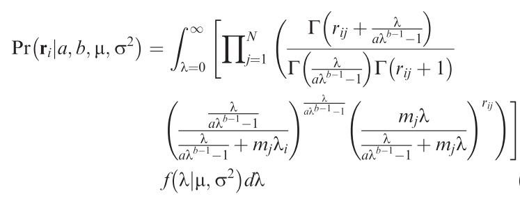
Analysis: Apply to one or more community data along a landscape structure gradient.

Requirements: Basic mathematics: The ugly function features all sorts of mathematical niceties, which at least require tolerance to formulae.

Time: The project can start anytime. Suitable as MSc project.

References: 

Connolly, S.R., Hughes, T.P. & Bellwood, D.R. (2017) A unified model explains commonness and rarity on coral reefs. Ecology Letters, 20, 477–486.

                                                                                                    >> Back to top